
By Dave Poole (Principal Data Engineer) and Daniel Durling (Senior Data Scientist)
Introduction to Snowflake Statistical Functions
Here at synvert TCM (formerly Crimson Macaw), as one of our preferred partners, we value the Snowflake statistical functions above and beyond traditional data warehouses.
To grow, a business needs a culture with a healthy attitude towards risk. That healthy attitude can be nurtured through an increased understanding of the organisation’s data and the use of statistical techniques to derive meaning from it. The ability to explain statistics in terms that a layperson would understand is key to building trust.
A robust statistical model supports such a culture by helping to understand the level of risk. This understanding can provide the illumination required for an informed decision where risk may be a consideration.
However, not only must the statistical model be a good fit for the subject it models it must be trusted as a good fit too.
This article is the first in a series where we look at how descriptive Snowflake statistical functions can help us understand our data.
- In Part 1 we look at some of the summary statistics functions that generate a single value.
- For Part 2 we investigate statistics which generate multiple values.
- And in Part 3 we combine our data and statistics with one of our recommended visualisation tools, AWS QuickSight, to show how visualising data can increase understanding.
Snowflake statistical functions
- COUNT
- SUM
- AVG
- MEDIAN
- MODE
- SKEW
- KURTOSIS
- STDDEV / STDDEV_SAMP
- STDDEV_POP
- VAR_SAMP / VARIANCE_SAMP
- VAR_POP / VARIANCE_POP
COUNT
The simple count gives us the number of rows within a table, which informs us of the size of the data we are looking at.
SUM
This arithmetic function will add values together.
AVG
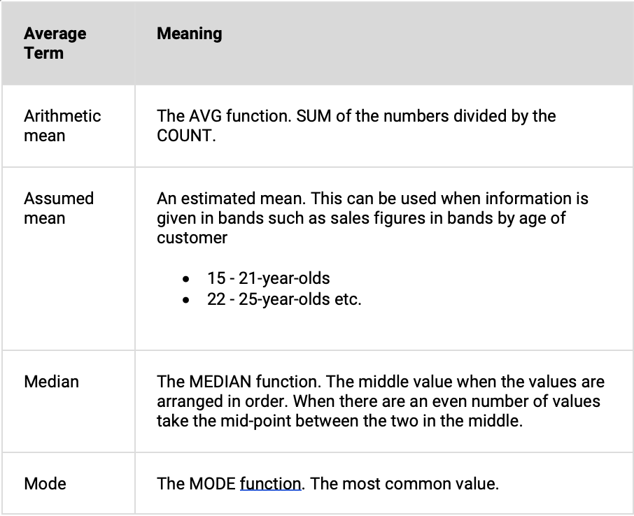
To the non-mathematical, an average is simply the SUM of the numbers divided by the COUNT. To a mathematician, this is called the “Arithmetic Mean”.
A mathematician/statistician probably won’t use the term “average” as an average is a generic term that can mean a variety of things. A statistician can use any of the terms below to mean average.
An average can even be a number picked at random within a range of values, though this is rarely used.
The problem with averages.
When we ask for the average customer what we are trying to do is describe typical customer behaviour.
Let us suppose that you want to know the average price of an item that a customer buys.
Take the example of a high-end hi-fi shop. A typical customer may buy a £2,000 amplifier and £100 of connecting leads. The average item spend is £1,050. But few customers buy at the £1,050 pricing point. Your average figure has little relevance!
To use an analogy, a man with his head in the oven and his feet in the fridge is, on average, perfectly comfortable.
Another example might be a market stall selling brushes and household knick-knacks. Prices range from £5 to £15, and all products sell equally well.
The average spend per item is £10. But there is nothing special about items costing £10! They sell equally well as items selling for £5 or £15. Plotting a graph of sales by unit price reveals a uniform distribution ().
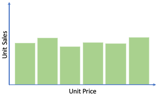
By itself, an average value is only useful if the values that you are measuring tend to cluster around that average.
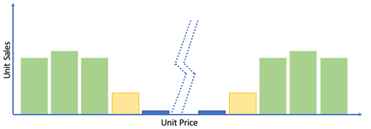
Catering for extremes
A further scenario is where values that are outliers or extremes distort the average.
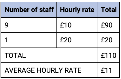
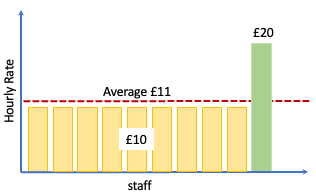
A single item is causing the average to be distorted upwards. 9 people will believe that they are underpaid rather than 1 being overpaid.
The AVG value is still useful, but we must consider the above issues when looking at it. We can gain more information from the AVG value when we use it in combination with the other average values.
MEDIAN
The median value is the number that represents the central point when those numbers are arranged in order.
If we look at our table of staff above the median value (the value that sits in the middle of the range) is £10.
Where there are an even number of values there will be no middle number. In this case, we take the average between the two nearest the middle of the list of values.
The median is not swayed by outliers as the mean is. This can be useful, but only if we are not too concerned with outliers.
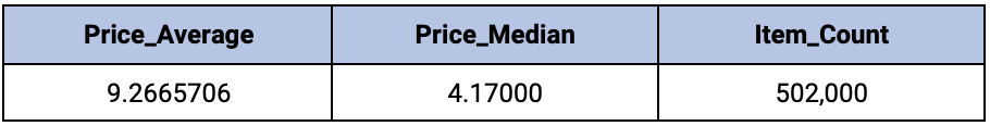
We can see an example of the average vs median scenario in the SNOWFLAKE_SAMPLE_DATA database.
SELECT AVG(i_current_price) AS Price_Average,
MEDIAN(i_current_price) AS Price_Median,
COUNT(*) AS Item_Count
FROM TPCDS_SF100TCL.ITEM;
This produces the results shown below.
MODE
The mode is the most commonly occurring value. The MODE always returns a real value from the data, rather than a calculated one. In our hi-fi example, this would highlight how different the most occurring value is from the MEAN.
Average interactions
We can use different averages together to get a fuller picture of the data we are looking at.
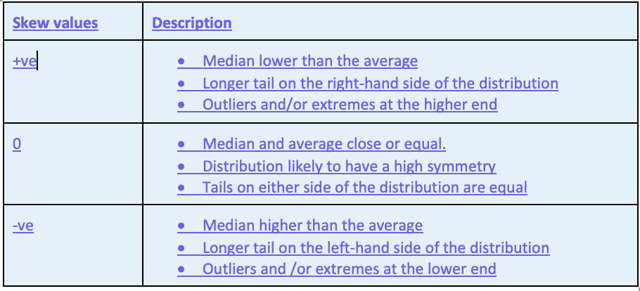
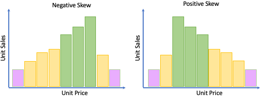
If the median is lower than the mean, then we can say the distribution is positively skewed, whereas if the median is greater than the mean then we can say it is negatively skewed.
If the mean is equal to the median and the mode, this implies a symmetrical distribution (but importantly it does not guarantee it).
VAR_SAMP, VAR_POP, STDDEV_SAMP & STDDEV_POP
How representative of the dataset is the mean? The VAR_SAMP, VAR_POP, STDDEV_SAMP & STDDEV_POP functions all give a single figure that describes how much the figures we are investigating deviate from our “average”. VAR_SAMP, VAR_POP both look to measure the Variance and STDDEV_SAMP & STDDEV_POP measure the Standard Deviation (of a sample and of a population respectively).
A quick aside on how a computer calculates variance and standard deviation
A point to make at this stage is that the way in which a computer or electronic calculator works out the VAR,VARP, STDDEV and STDDEVP is an approximation.
Let us take VARP as an example
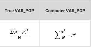
An explanation of the symbols is as follows:
- Σ = Sum
- x = A number in our range
- μ = The arithmetic mean (average)
- N = The number of numbers
The difference in the results between these two formulae is too small to be of much concern.
The reason the computer version of the formula is different dates to the days when computers were considerably less powerful than they are today. Basically, in the computer version of the formula, you can calculate your VARP in one pass through the record set, whereas in the true version, you would need to first calculate your average on one iteration, and then calculate your VARP on the 2nd iteration.
Variance
The variance is calculated as the squared difference of the values in the dataset from the mean. The bigger the number, the more spread out the values are from the mean.
The difference between VAR_SAMP and VAR_POP
The table below shows the difference between the two functions from a mathematical perspective
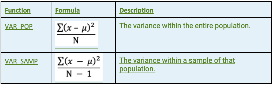
Let us suppose that it is not possible to measure the variance of an entire population. We would take a representative sample of that population and measure that instead.
If we were taking a sample, then wouldn’t we expect to build in some factor to allow for discrepancies in our sample?
Of course, we would. That is why the two functions have differing denominators (bottom half of the fractions).
As with any fraction, the bigger the denominator the smaller the eventual number so as we increase our sample size so the differences between what the functions return become smaller.
Standard Deviation
The Standard Deviation is the square root of the Variance, therefore:
- STDDEV_SAMP is simply the square root of VAR_SAMP
- STDDEV_POP is simply the square root of VAR_POP
Both the Variance and Standard Deviation can be represented by the Greek symbol Sigma
- σ = Standard deviation
- σ2 = Variance
The Standard Deviation is often more useful than the variance because the standard deviation is in the same unit as the data it is derived from. This becomes even more useful when we look at distributions in part 2.
Using Standard Deviation to understand the mean
The standard deviation provides statisticians with a very useful tool. For example, let us go back to the scenario where it is not possible to work with the full dataset and are therefore working with a sample.
If you take the average of your sample, you must also allow for some variability between the average of the population and the average of your sample.
In statistics, there is a term for this called the standard error of the mean. and this has a formula as follows

Let us suppose that we have a sample of 10,000 with an average of 5 and a standard deviation of 0.5.
Our standard error of the mean would be 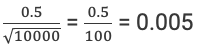
This means that from our sample we know that the true average within the population could be expected to fall +/-0.005 of our sample average of 5, or in other words between 4.995 and 5.005.
Skew
The SKEW value can be considered a measure of symmetry in a distribution. The closer to zero the more likely that the distribution is symmetrical.
Because of the caveats needed when looking at the skew, it is important to not look at it in isolation.
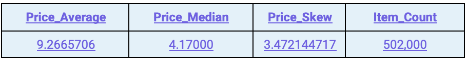
By adding the SKEW function to our earlier query, we can see that the prices in the ITEMS table are strongly distorted by high price items
SELECT
AVG(i_current_price) AS Price_Avg,
MEDIAN(i_current_price) AS Price_Median,
SKEW(i_current_price) AS Price_Skew,
COUNT(*) AS Item_Count
FROM  TPCDS_SF100TCL.ITEM;
This produces the results shown below.
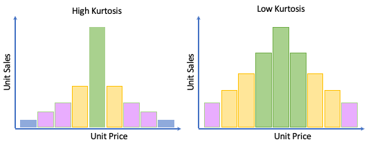
Kurtosis
The final single value function we are going to look at is KURTOSIS, which can be thought of as a measure of the length/weight of the tails of a distribution or can be thought of as an indicator of the presence of outliers in your data. The higher the Kurtosis score, the more certain you can be of the presence of outliers (values which are very far from the mean).
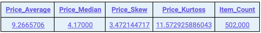
SELECT
AVG(i_current_price) AS Price_Avg,
MEDIAN(i_current_price) AS Price_Median,
SKEW(i_current_price) AS Price_Skew,
KURTOSIS(i_current_price) AS Price_Kurtosis,
COUNT(*) AS Item_Count
FROM  TPCDS_SF100TCL.ITEM;
This produces the results shown below indicating that there are highly likely to be extreme values present.
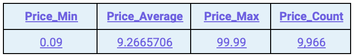
We can also see this when comparing the average item price to the minimum and maximum prices and the number of prices available.
SELECT
MIN(i_current_price) AS price_min,
AVG(i_current_price) AS Price_Avg,
MAX(i_current_price) AS Price_Max,
COUNT(DISTINCT i_current_price) AS Price_Count
FROM  TPCDS_SF100TCL.ITEM;
Understanding non-integer numbers
We know that the i_current_price column has a data type of NUMBER(7,2). With a price range of 0.09 to 99.99 and 9,966, we know we have items at almost every price point in between.
What would we do to assess the range of a more wide-ranging non-integer data type? This is where we can use Snowflake’s LOG function.
For any number, we know that 1 + LOG(10, number) will give us the number of digits to the left of the decimal place. The query below will tell us the number of digits in the fractional part of a decimal number.
SELECT
MIN(1+FLOOR(LOG(10,reverse(
CASE WHEN i_current_price % 1 = 0 THEN 1 ELSE i_current_price END
)))) fewest_decimal_places,
MAX(1+FLOOR(LOG(10,reverse(
CASE WHEN i_current_price % 1 = 0 THEN 1 ELSE i_current_price END
)))) most_decimal_places
FROM TPCDS_SF100TCL.ITEM;
The results are as follows

The query works by flipping a decimal number about the decimal point.
- 3.14 becomes 41.3
- LOG(10, 4.13) = 1.615950052
- 1+FLOOR(1.615950052) = 2.
The CASE statement caters for integer values which would otherwise give strange results.
- 200 becomes 0.002
- LOG(10,0.002) = -2.698970004
- 1+FLOOR(-2.698970004) = -2. A nonsensical value
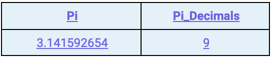
To show the methodology at work
SELECT
PI() AS Pi,
1+ FLOOR(LOG(10,REVERSE(PI()))) AS Pi_Decimals;
The results are as follows
Snowflake Statistical Functions: Conclusion
Hopefully, you have found our introduction to Snowflake statistical functions useful. That concludes part one of our tour of some of the most useful statistical functions contained within Snowflake. As you can see these single-value output functions can be very useful in isolation, but they are even more powerful when combined. In Part 2 you will see how we can combine them with even more functions to help you better understand your data.